|

Learn how to use Google forms and Google scripts to assist you in
|
|

|
|

|
|

|
|

|
NOW KNOW THIS...
|
|

|

|

|
FRONT END
|
1. You should now be looking at the front end of the document you copied into your Google Drive. You should NOT be looking at David's front end. Shame on you!
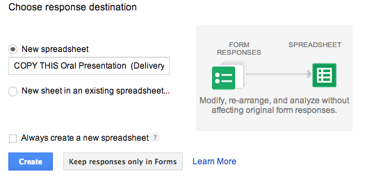
Anyway, this is your form in edit mode. It should look like this: 
2. You will now set up the form's back end to collect form responses. Click "Choose Response Destination."
2. Click "Create." Leave the default settings alone.
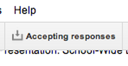
3. Don't click on this, but you should see that the form now indicates that it is accepting responses.
|
|


EVEN MORE
|
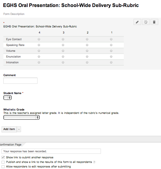
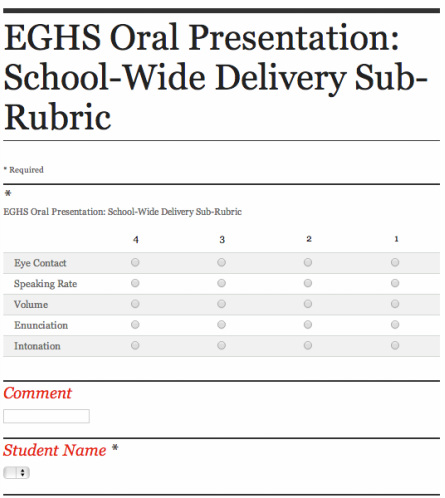
1. You should still be looking at the front end of your form in edit mode. It should look like this:
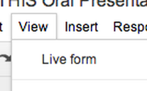
2. In a moment, you will fill out the form yourself. This will insure you have data to work with later. To open your live form do this: click View --> Live Form.
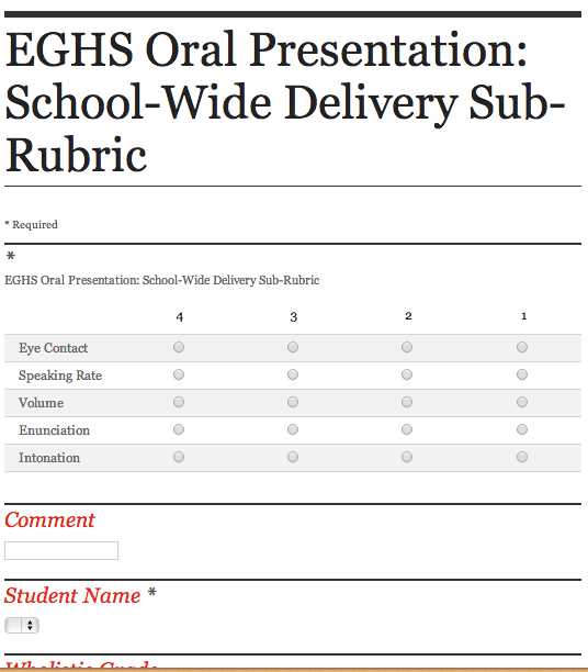
3. After opening your live form, you should see this:
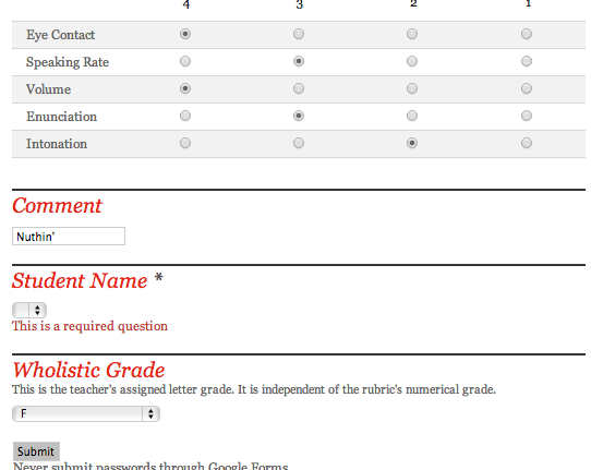
4. Fill out your form once. Click any number for each of the rubric items. Fill in anything you want under comment. Leave the student name blank for now. Select any holistic grade you like. Click submit.
|
|


THE BACK END
|
1. Now that you have submitted the information using your form, it's time to see the back end where this information lives. But first, you must leave the live form and return to the front end in edit mode. To do this, click on the tab in your browser where you were previously. They should look something like this:
2. Under the menu, you'll see an option to view responses. Click on "View Responses."
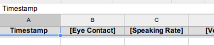
3. You should now see a spreadsheet that looks similar to this. You are now in the back end of your form. Notice that the information you entered into the form's front end is now stored in this spreadsheet.
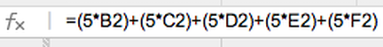
4. Next, you'll want to create a formula to tally the rubric grade. Click on the cell J2 to activate it. Click on the formula-box in the spreadsheet's top left corner. Copy and paste the following formula in the formula-box for cell J2: =(5*B2)+(5*C2)+(5*D2)+(5*E2)+(5*F2)
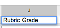
5. Press enter. You should see cell J2 automatically calculate a numerical grade based on the rubric scores you entered. If it doesn't, you probably forgot to copy the equal sign. Or maybe you copied the equal sign twice. Take another look at step 4 and try again. 6. Now, click on the cell, J1. Name cell J1 Rubric Grade by typing the words Rubric Grade in the cell.
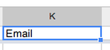
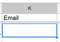
7. Click on the cell, K1. Name cell K1 Email by typing the word Email in the cell. Press enter. Leave that column empty otherwise for now. We'll revisit it later.
8. Look down at the bottom left side of the sheet. Click the plus sign to add a new sheet. You should see a new tab called Sheet2. Double click on the word, Sheet2. Change the new sheet's name from Sheet2 to exactly Student Name Email by typing over the word, Sheet2.
13. Click on K2, which is the first empty cell in the Email column.
14. In the formula box for cell K2, copy and paste this formula exactly: =VLOOKUP(H2,'Student Name Email'!A:B,2,FALSE)
NOW YOU'VE GOT IT... 
NICE! You are now in a great place. Your form is all prepped and ready to go for some automagical Google scripts...
|
|


SCRIPTS
|
A script can automate repetitive tasks for you. We'll use three today:
|
